
(Original image by Hljod.Huskona / CC BY-SA 2.0).
I used to hate neural nets. Mostly, I realise now, because I struggled to implement them correctly. Texts explaining the working of neural nets focus heavily on the mathematical mechanics, and this is good for theoretical understanding and correct usage. However, this approach is terrible for the poor implementer, neglecting many of the details that concern him or her.
This tutorial is an implementation guide. It is not an explanation of how or why neural nets work, or when they should or should not be used. This tutorial will tell you step by step how to implement a very basic neural network. It comes with a simple example problem, and I include several results that you can compare with those that you find.
I tried to make the design as straightforward as possible. The training algorithm is simple backpropagation. There are no hidden layers (I will treat that in an upcoming tutorial), no momentum, no adaptive learning rates, and no sophisticated stopping conditions. Those are, in a sense, easy to add once you have a working neural net against which you can benchmark more elaborate designs.
To keep the implementation simple, I did not bother with optimisation. This too can easily be addressed once a working neural net is in place against which you can verify correctness and measure performance improvements.
The brief introduction below is a very superficial explanation of a neural net; it is included mostly to establish terminology and help you map it to the concepts that are explained in more detail in other texts.
Preliminary remarks and overview
What we are doing
The problem we are trying to solve is this: we have some measurements (features of an object), and we have a good idea that these features might tell us in which class the object belongs. For example, if we are dealing with fruit, knowing the size, colour, and “roughness” of the skin, we might deduce which type the fruit is. Of course, we want a program for this.
Now in heaven, there is a function for exactly that task – we give the function the features, and it spits out the class.
Down here on earth, we are not so lucky (well, not for most problems anyway). So instead, we have to do with some approximation. A neural net is one possibility – there are also others. A neural net (one without any hidden layers) is parameterised by a weight matrix. Different problems in general have different weight matrices. To solve our problem, we need to find a suitable matrix.
If both our set of known samples and the problem itself are reasonable, we might expect to find such a matrix. But not directly – we have to use some kind of iterative scheme – we have to “train” our neural net. We use some of the known samples for this.
Behind the scenes, the weight matrix and the feature vector are combined using some matrix operations to give the output vector, which is converted to a class. The mathematical details of this can be found elsewhere (more).
After we have trained the neural net, we can use it in an application to classify objects that we may or may not have encountered before. Generally, the training and application programs are separate. The training program is the difficult part; most of the tutorial deals with training.
It is common to divide the known samples in three sets, called the training set, validation set, and test set, typically divided in the ratio 50%, 25%, and 25%. The training set is used to update the weights iteratively; the validation set is used to stop the training algorithm, and the test set is used to estimate how well our trained neural net will do in the wild.
Each iteration of the training algorithm is called, quite poetically, an epoch. Many different things affect the number of epochs we will need to train the neural net: the problem complexity, how we scale our updates, and how the weight matrix has been initialised.
We can control the speed with a parameter called the learning rate. In general, higher learning rate means faster learning (although, when it is set too high, the network might become unstable and not learn at all).
Representation
We usually represent the features (our measurements) as a vector of numbers, like this:
[0.01, 1.07, 3.60]
In cases of non-numeric values, we convert whatever we have to numbers with some scheme. For instance, when dealing with colours, we might want to use RGB values, or we might want to make a list of colours (red, yellow, green, etc.), assign a number to each of these labels, and use the corresponding number.
Classes, usually not being numbers, are similarly treated: we assign a number (often arbitrarily) to each class, and use that in our computations. For the actual training, however, we use an output vector. The output vector has a 1 in the position of the class number, and 0 everywhere else.
Thus, if we are dealing with three classes of fruit (apple, pear, banana), and number the classes 1, 2, and 3 respectively, we will have the following output vectors:
| Class | Class Number | Output Vector |
| Apple | 1 | 1 0 0 |
| Pear | 2 | 0 1 0 |
| Banana | 3 | 0 0 1 |
It is convenient to put all the inputs of a set together in a single matrix, where each row is a sample. Similarly, outputs and classes are also put into matrices, with input sample in a row (say row number n) corresponds to output sample in row n, and also the class in row n.
The implementation below makes use of high-level matrix operations. This avoids many of the errors that can creep in loop-dense code. The following table will give dimensions of all the matrixes involved; this will be helpful during implementation (especially for assert statements). The numbers are given in terms of the number of inputs (features) of the problem, the number of outputs.
| Matrix | Rows | Columns |
| input vector of a single sample | 1 | input_count |
| output vector of a single sample | 1 | output_count |
| class vector of a single sample | 1 | 1 |
| input matrix of training set | training_count | input_count |
| output matrix of training set | training_count | output_count |
| class vector of training set | training_count | 1 |
| bias vector of training set | training_count | 1 |
| net vector of single sample | 1 | output_count |
| weights matrix | input_count + 1 | output_count |
| weights delta matrix | input_count + 1 | output_count |
| error vector | 1 | output_count |
| delta (sensitivity vector) | 1 | output_count |
Overview
The basic idea of the training algorithm is the following:
First we load in the data: the training samples, the validation samples, and the test samples.
Then we start to train: we run the backpropagation algorithm on random samples. After each iteration, we see how our network is doing so far (on the validation set), and then we decide whether to keep training or not.
After we stopped, we do a final evaluation of our network on the test set – this gives us an indication of whether the neural net will generalise well to samples not originally in the training set.
After we have found a weight matrix that we can live with, we cfan incorporate this in the application were we need the functionality.
The training program has x functions:
- train
- load data
- feed-forward
- evaluate network
- backpropagation
- output to class
- class to output
- activation
- activation derivative
The application program uses these functions:
- feed-forward
- output vector to class
Implementation
1. Gather the necessary libraries (or write them)
You will need the following libraries:
- A library that supports matrix algebra; and
- A library that plots graphs (x versus y).
If you can’t find a matrix library for your implementation language, then you can write a simple library yourself. Since neural nets do not require matrix inverses or long chains of matrix products, you need not worry (much) about numerical stability, thus the implementation is straightforward.
The implementation needs to support the following matrix operations:
- matrix transposition;
- matrix addition;
- matrix multiplication with a scalar;
- ordinary matrix multiplication;
- Hadamard multiplication (component-wise multiplication);
- Kronecker multiplication (only necessary for between row and column vectors); and
- horizontal matrix concatenation.
The first few operations are standard matrix operations, but you might be less familiar with the last three. (Also check out the Wikipedia article on matrix multiplication – it covers all the types of multiplication mentioned here.)
Hadamard multiplication of matrices is defined for two matrices of equal dimensions. Each component of the new matrix is the product of corresponding components in the two multiplicands, that is:
Z[i][j] = X[i][j] * Y[i][j]
The Kronecker product of a row vector and column vector is defined as a matrix whose components are given by:
Z[i][j] = X[0][i] * Y[j][0]
It is possible to define the product for arbitrary matrices, but we don’t need it.
The horizontal concatenation combines two matrices with the same number of rows. For example, the matrices A and B below will be concatenated to form the new matrix C:
A=\begin{pmatrix}10 & 3\\4 & 5\end{pmatrix},\:B=\begin{pmatrix}6 & 8 & 2\\3&1&10\end{pmatrix},\:C=\begin{pmatrix}10 & 3&6 & 8 & 2\\4 & 5& 3 &1&10\end{pmatrix}
A simple implementation simply constructs a new matrix whose components are given by
if j < X_width
  Z[i][j] = X[i][j]
else
   Z[i][j] = Y[i, j – X_width]
If no graph libraries are available, simply write a function that will output a tab-separated list of the input and output sequences to plot. You can then load or paste this into your favourite spreadsheet program to make the necessary plots.
2. Implement Output and Class conversion functions
This is very simple: implement a function that converts an output matrix to a class number vector, and another that converts a class number to an output vector.
For example, the output_to_class function will take the following matrix
1 0 0
0 1 0
0 0 1
1 0 0
0 0 1
and convert it to:
1
2
3
1
3
(The second function will convert the second matrix back to the first matrix).
3. Implement a function to read in data files
For this tutorial you can use the following three files:
- iris_training.dat
- iris_validation.dat
- iris_test.dat
These three files contain samples from the ICU iris dataset, a simple and quite famous dataset. In each file, samples or contained in rows. Each row has seven entries, separated by tabs. The first four entries are features of irises (sepal length, sepal width, petal length, and petal width); the last three is the outputs denoting the species of iris (setosa, versicolor, and virginica). I have preprocessed the values a bit to get them in the appropriate ranges.
You must read in the data so that you can treat the inputs of each set as a single matrix; similarly for the outputs.
I find it useful to store all the data in a structure, like this:
- data_set
- input_count
- output_count
- training_set
- inputs
- outputs
- classes
- count
- bias
- validation_set
- inputs
- outputs
- classes
- count
- bias
- test_set
- inputs
- outputs
- classes
- count
- bias
This makes it more useful to send the data as parameters.
4. Implement an activation function and its derivative
The activation function must take in a matrix X, and return a matrix Y. Y is computed by applying a function component-wise to X. For now, use the hyperbolic tangent function:
f(x) = \dfrac{\tanh(x) + 1}{2}
The activation function derivative must similarly take in a matrix X, and return a matrix Y. Y is computed by applying the derivative of the activation componentwise to X. The derivative of the function above is:
$latex f'(x) = \dfrac{1 – \tanh^2(x)}{2}$
5. Implement the feed-forward function
The function must take as arguments an input matrix, weight matrix, and a bias node matrix.
The function should return an output matrix, and a net matrix
These are computed as follows:
net = mul(weights, horcat(inputs, bias))
output = activate(net)
The bias matrix is a constant column vector of 1s with as many rows as the input matrix. This vector corresponds to the bias nodes. The implementation here is a bit clumsy, but for now, the approach used here minimises the potential for error.
6. Implement a weight initialisation function
This function must take in a maximum weight, a width and height, and return a matrix of the given width and height, randomly initialised in the range [-max_weight max_weight].
7. Implement a function that evaluates the network error.
The function must take in:
- an input matrix,
- a weight matrix,
- a target output matrix,
- a target class matrix,
- a bias matrix.
The function must return the error e, and the classification error c.
To compute these, first compute the output matrix Z using the feed-forward function (you can ignore the net matrix).
[output net] = feedforward(inputs, weights, bias)
Now subtract the target output matrix from the output matrix, square the components, add together, and normalise:
error = sum_all_components((target_outputs – outputs)^2) ...
/ (sample_count * output_count)
From the output matrix, calculate the classes:
classes = classes_from_output_vectors(outputs)
Count the number of classes that corresponds with the target classes, and divide by the number of samples to normalise:
c = sum_all_components(classes != target_classes)/sample_count
(Here, our inequality returns a matrix of 0s and 1s, with 1s in positions where the corresponding components in classes and target_classes are not equal.)
8. Implement a dummy backpropagation function
The function should take in:
- An input matrix
- A weight matrix
- a learning rate (eta, as in the Greek letter)
- a bias vector
The function must return an updated weight matrix. For now, return W as is.
9. Implement the train function
The training function should take in three sets, the training_set, validation_set, and test_set. Implement a way to limit the maximum number of samples that will actually be used for training (you can also do his in the main program described in the next section). This is very helpful for debugging purposes (especially if you plan to later replace the backpropagation algorithm with something a little faster – and more complicated).
The function should return a weight matrix, and error values as floats.
Initialise a value plot_graphs to true. This is a debug flag, so it is appropriate to implement this as a macro if it is supported by the implementation language.
The function should initialise a weight matrix using initialise weights. For now, use a max_weight of 1/2.
The function should also construct three bias vectors bias_training, bias_validate, and bias_test. Each must contain only 1s, with as many rows as there are inputs in the training, validation and test sets respectively.
Implement a while loop that stops after 500 iterations. (We will change the while condition later to something else, so do not use a for loop).
Inside the loop, call the backpropagation algorithm. Use the training set inputs, the weights, (for now) a fixed learning rate of 0.1, and bias vector bias_train. Assign the result to weights.
Still inside the loop, call the network error function three times: one time for each of the training, validation, and test sets. Use the weight matrix, and the appropriate bias vector. Wrap these calls in an if-statement that tests for a value plot_graphs. (If your language supports it, you can use conditional compilation on the value of plot_graphs).
Store the errors in six arrays (error_train, classification_error_train, etc.), with the current epoch number as index.
After the loop, plot the six error arrays as a function of epoch number. Wrap this in an if-statement (or conditional compilation statement) that tests for the value plot_graphs.
Call the network error function again, on all three sets as before.
Return the weights, and the six errors.
10. Implement the main training program
The program should load in the sets (using the load_sets function), and pass these to the training algorithm.
11. Run the program
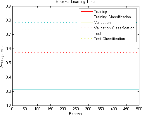
The important thing is that everything should run. You should see your error plots; at this stage they should be straight, horizontal lines. Because of the random weight initialisation, we cannot predict where these lines will lie (so do not be alarmed if they do not look exactly the same as below – as long as they are straight and horizontal).
12. Implement the backpropagation function
You have already created the dummy function; now you can put in the actual calculations.
First, select a random sample.
Now, calculate the net matrix and output matrix using the feed-forward function.
[output, net] = feedforward(random_sample, weights, bias)
Calculate the error vector
error_vector = target_outputs - outputs
Calculate the sensitivity.
delta = hammard(error_vector, activation_diff(net))
The corresponding mathematical expression in the textbook might look like this:
\delta_k = (t_k - z_k) f'(y_k)
Calculate the weights delta:
weights_delta = scalar_mul(eta, kronecker(transpose(outputs), delta))
The corresponding mathematical expression in the textbook might look like this:
w_{kj} = \eta (t_k - z_k) f'(y_k)y_j
Update the weights:
weights = add(weights, weights_delta)
and return the matrix.
13 Run the program (AGAIN)
First, set the debug option to train on only one sample. The curve should like like this:
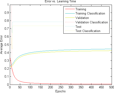
Notice that the error curves are smooth, the training error rate goes to 0, and the other error rates go to 0.4, plus or minus – this depends on the initial weights. It will also be different if you use a sample other than the first.
If your curve looks right, change the debug option to train on all samples. Your error curves should now look something like this:
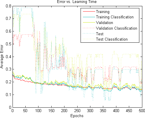
The important feature of the error curves is that they should steadily descent on average. If your curve does not resemble the one shown here; there is a mistake in your implementation. It is often helpful to limit the training set to a single sample (thereby eliminating the randomisation of sampling during training) to see what is going on.
Although the errors often follow the relationship training < validation < test, this is not always the case, so do not be alarmed if this is not true on a run (You can see it is not always true in the run above).
14 Implement a proper stopping condition
Change the while loop to stop when the validation error drops below a threshold. Note that this threshold usually depends on the problem. There are better stopping conditions that are less sensitive to the problem at hand, but this one will do for now.
15 Implement a statistical analysis
This part is important for you to get an idea of the robustness of the neural net. In practice, a very simple analysis will suffice.
This part need to train the algorithm 30 times, and then report the mean, standard deviation and maximum of the
- training time,
- regression error, and
- classification error (on the test sets).
In general, you would like all these values to be “low”. Here are some experiments for the iris data set with different learning rates. For each, 30 runs were made; other parameters are as described earlier (max_weight = 1/2, validation_stop_threshold = 0.1).
| Mean | Standard Deviation | Maximum | |
| eta = 0.05 | |||
| Training time | 1200 | 124.681 | 1489 |
| Regression error | 0.115343 | 0.0017233 | 0.11894 |
| Classification Error | 0.17807 | 0.0456762 | 0.263158 |
| eta = 0.1 | |||
| Training time | 582.533 | 65.3076 | 719 |
| Regression error | 0.114626 | 0.00180851 | 0.118697 |
| Classification Error | 0.214912 | 0.0317323 | 0.263158 |
| eta = 0.5 | |||
| Training time | 120.967 | 16.7095 | 169 |
| Regression error | 0.115711 | 0.0038786 | 0.123573 |
| Classification Error | 0.245614 | 0.0242702 | 0.263158 |
| eta = 1 | |||
| Training time | 67.1667 | 12.2477 | 99 |
| Regression error | 0.114755 | 0.00488566 | 0.124468 |
| Classification Error | 0.253509 | 0.0201287 | 0.263158 |
Using the neural net in a program
To use the neural net in a program after you have trained it, you need to save the weights found by the training program to a file. Your application must then read in this weights, and use it with the feedforward function to calculate the class.
Here is pseudo-code for the program. Note that the training program and classification program needn’t be implemented in the same language. This allows you to take advantage of speed and interface components that might not be available in your target platform. It is a very good idea to implement your training algorithm on a computer algebra system (such as Matlab or Octave) where you can take advantage of both matrix and graphing capabilities (the code provided below works in both).
Using the training algorithm on other problems
When using your neural net for other algorithms, you might need to change the learning rate, stopping threshold, and weight_max for weight the initialisation. The error plots are indispensible for this purpose.
As long as the learning rate is not too high, it should not affect the quality of the solution, only the number of iterations necessary to obtain it. The stopping threshold, however, has does affect the quality of the solution: if it is tool low, the problem might not be solved, or the neural net might train very long; if it is too high, you will get poor performance. There are better stopping conditions available; once you have everything working, you should investigate these.
Remember that you should not base your decisions on a single run, as runs can differ quite drastically from one another. Perform a few runs, and base decisions on these.
The value weight_max can usually be chosen as 1/sqrt(input_count) with good results, but here too it depends on the problem.
For further benchmarking, check out the Proben1 datasets, described here. (Also check out the erratum note on this site – search for proben on the page.)
Download
The following code works in Matlab and Octave. (Included is a randint function; if you are using Matlab you can remove it, because it is already implemented in Matlab).
iris_data_files.zip (3 KB)
basic_neural_net_0_1.zip (10 KB)
The program provided cheats a little – instead of reading in the raw .dat files, it reads in the .mat file that already has the data in the right structure.

Hello, im implementing a back propagation algorithm for neural network on matlab, i would like to know if you have or know about links or books about the mathematical aspects of the algorithm (The mathematical details of this can be found elsewhere.<—– link doesnt work ) and i would like to know de details of the matrix algebra used.
thanks in advance
Mario,
Thanks for spotting the broken link; it is fixed now 🙂
The Neural Networks Chapter in Pattern Recognition (http://www.amazon.com/Pattern-Classification-2nd-Richard-Duda/dp/0471056693) is also decent, although the math there is not written out in as much detail as it could be.
ht
Just a correction, im Mario =P, thanks for the information
:”> fixed…
Hi i would like to have the coding for differentiation of fruits using back propogation algorithim.. Its for my finall year project
Hi there,
thanks for your information on neural networks – it has been of great interest.
regarding the output of networks, up until this point, i have only ever seen networks or examples which give either a binary output, or a continuous output bounded between 0 – 1 …
i am looking at using a NN to predict machine efficiency based on a number of input parameters, and would like an output of say between 0 – 100%. i know this can be represented as 0 – 1, however, the point would be to use unbounded real numbers in order to allow for prediction of perhaps other parameters as well, such as lengths in mm etc.
Are you aware of how this can be handled with MLP’s or perhaps shed some light based on your own experience?
many thanks
jon
It is an excellent implementation example. I loved it. Has the author written hidden layers also?
Good One… Thank You
Great guide, thanks! Just one question.. In step 7, in the function for evaluating the network error, you write that we should subtract the target outputs from the outputs returned by the feed-forward algorithm.
However, as I understand, the target outputs are going to be a matrix of height = sample_count and width = 3 (for the 3 possible classifications of the iris dataset).
The result from the feed-forward algorithm, though, is a matrix of height = sample_count and width = 5, because as it is described in step 5, we form the output matrix to return by concatenating a vertical bias vector horizontally to the input matrix of width 4 (sepal length/width, etc).
Am I misunderstanding what you mean by “target output”?
Thanks in advance for your advice.
I’ve had the same question, as to what is meant by “target class matrix” and “target output”. Is the “target class matrix” obtained from the last element of each of the rows read from the file? Or is that the “target output”?
@tylerklement:disqus have you managed to clarify your initial question? I am also stuck here.
Thanks for your time,
Pedro
@tylerklement:disqus Have you found an answer for this? I am also stuck here. Are we following it wrong to get two matrices with different dimensions when subtracting. My error stems from the fact that “target_output_matrix” has dimensions of (75,3) where “output_matrix” produced from the feed-forward has dimensions of (75,5). Do we need to lower the dimensions of it? Or did I follow the steps incorrectly?
Thanks for your time,
Pedro
Hello all…I can find data file “mushroom”…
The site looks great, I download the files and can not execute them because the first thing that training_main_app does is loading (‘mushroom1’)…
thank you …
Could you find what is Mushroom file exactly ? I tried giving dat files as input, but its not working…
Change mushroom1 to iris1
Yes the matlab code doesnt work..
This looks like a nice guide! But what does `activation_diff(net)` mean? Does it mean derivative function? Thanks in advance.
In the sample code, [inputs, bias] * weights on the feedforward function, but the reading above implies weights * [inputs, bias]. Awesome implementation, btw!