A cellular automata system is one of the best demonstrations of emergence. If you do not know what cellular automata (CA) is, then you should go download Conway’s Game of Life immediately:
Essentially, CA is a collection of state machines, updated in discrete time intervals. The next state of one of these depends on the current state as well as the states of neighbours. Usually, the state machines correspond to cells in a grid, and the neighbours of a cell are the cells connected to that cell. For a more detailed explanation, see the Wikipedia article.
Even simple update rules can lead to interesting behaviour: patterns that cannot be predicted from the rules except by running them. With suitable rules, CA can simulate many systems:
- Natural phenomena: weather, fire, plant growth, migration patterns, spread of disease.
- Socio-economic phenomena: urbanisation, segregation, construction and property development, traffic, spread of news.
In games, these can be used as game elements (such as fire and disease), or they can also add some decorative life to a game (such as city development in a simulation game).
The great thing about CA systems is that they are not hard to implement, and they have intrinsic fun value (I mean here, for the programmer!).
Before we get into the details, let me add a small disclaimer here:
- This tutorial is not comprehensive. I only touch on a few ideas in a wide field. See some of the resources at the end for more information.
- This tutorial is not representative. I merely chose topics I found interesting or thought would be useful for game developers.
- I am not suggesting that using cellular automata is the best way to simulate any of the examples given here. For any problem, there might be solutions that are faster, easier to implement, or yield better results.
Implementation
To implement a CA system, you need to do the following:
- Use a suitable system to store states, for example, a 2D array.
- Decide on a suitable neighbourhood shape, and work out some preliminary rules. Decide how you will handle edges.
- Implement a suitable way to describe your rules.
- Implement an update function that hooks into the main game loop.
- Implement a visualisation scheme (for example, drawing tiles depending on states in the array).
Some details of these are described below.
Grid
A typical implementation uses two grids for storing states. One is the current world state; the other is the new world state. Once all cells have been updated for the current iteration, pointers to the arrays can be swapped. This way updating the cells one by one will not have an effect on other cells until the next iteration, and you do not have to create a new array in each iteration.
Using grids with square cells are the easiest to implement, but the concept is also applicable to other grids: hexagonal and triangular grids are also common, and even polar grids have been used to simulate spiral star systems.
It is also possible to use irregular systems, although the implementation then becomes a challenge. One example of an irregular system is a presentation based on a Poisson distribution of points. The trick here is to find an efficient way to locate neighbours. Fortunately, this problem has already been solved in creating the points (see the Poisson Sampling tutorial in Dev.Mag). It is in fact done by using an invisible grid! Of course, visualising a state is also a bit more difficult.
Neighbourhoods
For 2D cellular automata, the most common neighbourhoods are the Von Neumann neighbourhood and the Moore neighbourhood, shown below (the blue cell’s neighbourhood is shown in red). Other neighbourhoods are also possible.
 |
 |
 |
| Von Neumann neighbourhood | Moore neighbourhood | Extended Von Neumann neighbourhood |
The cell can be included in the neighbourhood or not. It is advisable to keep the neighbourhoods as small as possible: not only does the neighbourhood size impact performance, it also affects the number of rules to be specified and thus the tweaking complexity.
Specifying Update Rules
Specifying the rules concisely is the most challenging part of implementing CA. With very simple models, you might want to use a few if/else statements. This, however, makes it hard to modify (tweak or extend), and is therefore not suitable for more complicated systems.
It is best to implement rules as a table that can be indexed using the neighbourhood states.
Table as an array. In this method, each row represents the combined state of the surrounding cells. The final entry in the row is the new state of the current cell. Each of the remaining columns represents a state. The entries in these columns represent the number of cells surrounding the current cell in that state.
| Dry Bush | Burning Bush | Charcoal | New State |
| 4 | 0 | 0 | Dry Bush |
| 3 | 1 | 0 | Burning Bush |
| 3 | 0 | 1 | Dry Bush |
| 2 | 2 | 0 | Burning Bush |
| 2 | 1 | 1 | Burning Bush |
| 2 | 0 | 2 | Burning Bush |
A cell surrounded with three cells in the Dry Bush state and one cell in the Burning Bush state will go into the Burning Bush state.
This table can be quite large, so that you must take care to implement lookups efficiently. Keep the table sorted, and perform binary search to lookup entries. Below are some improvements on this scheme.
Table as a tree. In the table above, it is easy to see that if there are three dry bush nodes, there are two possibilities for the other states (either 1 0, or 0 1). We can use this to implement a tree. Each level in the tree represents a state. A value in a node represents how many cells in the neighbourhood are in that state. A path from root to leaf fully describes the states of the entire neighbourhood. We do not add nodes for the last state, as it is uniquely determined by the other states.
Below is a tree corresponding to the piece of table above.
BB = Burning Bush
DB = Dry Bush
| root | +— | DB 4 | DB | ||
| +— | DB 3 | +— | BB 1 | BB | |
| | | +— | BB 0 | DB | ||
| +— | DB 2 | +— | BB 2 | BB | |
| +— | BB 1 | BB | |||
| +— | BB 0 | BB |
This is a more efficient implementation; unfortunately, it is also more complicated. It is inconvenient to specify the tree in a tree-friendly format (XML or s-expressions, for example). You still need to specify it in table format (space separated text file, for example) and build the tree from that.
Implementation as a hash table. Here you use tuples of state counts as keys. For example, the third entry in the table above can be accessed with the tuple (3, 0, 1). If your implementation language does not support tuples, you might need to implement them yourself. Be sure to make them immutable!
Implementation as an N-dimensional array. This is a very simple method, although it wastes a lot of memory. N is the number of states, and we use the state counts to index into the array. In our example, we will use a 3D array, so that the third element can be accessed using transition_array[3, 0, 1].
The method above can be used even when the implementation language does not provide N dimensional arrays. Simply use a 1D array, and interpret the state counts as the digits of a base-4 number. Thus, the third row will be located at 3*16 + 0*4 + 1*1 = 49.
Note that since the numbers are restricted by the requirement that they add to four, there will be unused array positions in both these last two methods. You can save memory by not using the last state to index (since it is uniquely determined by the other states). Thus, we can use a 2D array, and access the 3,0,1 rule with 3,0 alone: transition_array[3, 0]. Alternatively, if we need to use a 1D array, we can store the rule in the position 3*4 + 0*1 = 12. Although the same scheme is possible for the hash table implementation, I would advise you to use the full indexing scheme instead, since it will not waste more memory if you do, and it is somewhat easier to understand if you use full indices.
Some rules do not need the detailed tables above. For instance, in a system of only two states, where transitions depend on the count of the states of the neighbourhood, we can use a simple array, indexed by one of the states’ counts. Many other schemes are possible: in general, aim for quick lookups and easy specification.
Edges
The edges of your simulation might present some problems: edges often serve as unwanted sources, sinks or stabilisers.
A source is the origin of outward growth (states change progressively to a specific state in an outward direction).
 |
 |
 |
 |
A sink is the exact opposite:
 |
 |
 |
 |
Sources and sinks are emergent properties of the CA system, and are not physical attributes of the cells.
 A stabiliser is a section that keeps neighbouring states fixed. For example, in the fire simulation (described below), there is an unnatural wall of fire around the edges at the end of the simulation.
There are several ways you can handle edges:
Ignore them. When the edge anomalies are acceptable, it is best not to complicate the model. This is only possible if the rules are specified in a way that does not require state counts to sum to the size of the neighbourhood. For example, if there is a rule “if num_states_fire > 1, then …”.
Wrap around. This solution is very elegant, easy to implement, and its effects are easy to understand. However, it is usually easy to see that the world has been wrapped in this way, and hence it is not always a visually a satisfactory solution. It is possible, however, to simulate a grid bigger than displayed area (say about double). This will hide the fact that it is wrapped, but still give you the benefits of having a world without any discontinuities.
 In the CA system shown left, we want to calculate the next state of the grey cell. Two neighbours fall outside the edges. If we wrap around, we use the four red squares as shown.
Reflection. Use a neighbouring state to perform calculations.
 The CA system shown left is the same situation as above. If we use neighbouring states for the cells beyond the edges, we use the state of the grey cell (twice!), in addition to the two red cells shown.
Fix their states. The edges can be given special, constant states that make the CA behave as intended. Finding the right state(s) for the edges might be difficult.
An implementation trick that applies to the last three edge-handling techniques is to include a border in your simulation. For the Von Neumann and Moore neighbourhoods, this border is only one cell thick.
This border is used for updates like all other cells, but is itself updated differently. The update rules for wrapping and reflection will simply copy states from the right places; the border for fixed states will never be updated.
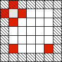 In the figure, hatched cells are updated according to the special rules of the edge-handling scheme – in this case, wrapping is used, so they are simply copied from the appropriate cells. All other cells are updated normally. Note that here we do not need special logic for updating the grey cell.
A Few Examples
(Also see the downloads at the bottom of the post).
Heat
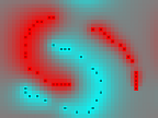 Here, continuous states (floats between 0 and 1) are used. Every cell is updated to a weighted average of its Moore neighbourhood cells: corners have a smaller weight than other cells. For this simulation, heat sinks and sources have been added: they keep the cell’s temperature at 0 and 1 respectively.
City Roads
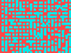 This simulation use separate neighbourhoods for creating and destroying a road. The creation neighbourhood is an extended Von Neumann neighbourhood; the destruction neighbourhood is a Moor neighbourhood. Creation and destruction is according to probabilities based on the count of neighbouring roads.
Influence
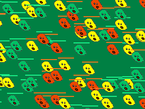
This simulation models human emotion as influenced by others. A character has an internal state, and an externally visible state. Characters can only observer the external state of their neighbours. The internal state is then a modified: a character surrounded by angry people will itself become angry, and so on. The external state is probabilistically determined by the internal state.
Disease Spread
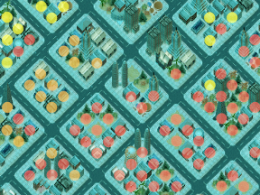 For our game Epidemic, Chris and I used a simple diffusion model. We used a floating-point number for the state, and represented the number of infected people in a cell. We used different colours for different ratios to visualise infection. At each time step, a cell would become infected by an amount proportional to that of the neighbourhood, with some random scaling.
Visualising States
Versions of tiles
A very effective way of making CA simulations more impressive is to have more than one tile for each state, and display them randomly. This is especially helpful for hiding regularity in off-line simulations. Tile sets with different versions for corners, edges, and central regions can drastically improve the look of the game, although it complicates choosing the correct tile version. In addition, it means you need tiles for various combinations of states. Assuming we can rotate and reflect tiles, in the fire example with three states, we need the following tiles:
| 3 centre tiles | |
| 3 straight-edge tiles | |
| 3 diagonal line tiles | |
| 3 cross tiles | |
| 6 corner tiles | |
| 3 half-straight tiles |
This is 21 tiles for only three states. It is advisable to automate tile creation.
Tile
States can be animated. Instead of displaying a single tile, display an animation sequence. You will need to think about how to start and stop these animations so that they are seamless. For instance, you can make all animation sequences the same length, and only update states between animation sequences.
You can also increase the seamlessness of the simulation by animating transitions between states. This can be as easy as blending between two tiles over a period of time (assuming that updates are made far enough apart).
No Tiles
Instead of using tiles to represent a state of a cell, you can put objects in a cell. For instance, in a plant growth simulation, you can put a number of trees in the cell depending on the state. The advantages of this are:
- You do not have to create dozens of tiles for variety.
- The player can interact with the objects. For instance, the plant placement of trees can hinder a player’s movement.
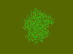
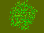
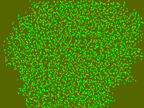
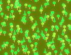 This shows a simple forest simulation. Trees grow and die depending on the surrounding trees. This system uses a grid, but not tiles: trees can grow in random positions in tiles. For this simulation, three random coordinates have been chosen for each cell at the beginning of the simulation. Depending on the states, one, two, or three trees will be drawn at these points. Choosing a fixed set of points makes it easier to draw trees at the same coordinates every tick. A somewhat more complicated simulation can choose new points whenever a new tree comes into being.
 |
 |
 |
CA Enhancements
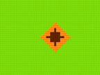
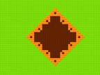
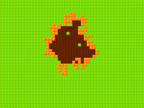
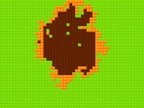
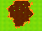
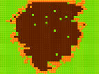
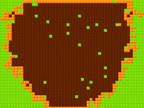
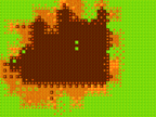
The images below show three frames from a simple fire simulation.
 |
 |
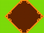 |
The green is grass (Dry Bush), the orange is fire (Burning Bush) and the brown is burnt grass (Charcoal).
As you can see, the simulation captures some features of a fire:
- fire grows outward,
- grass only burns once,
- grass needs fire to catch fire (there is no spontaneous combustion).
Even so, the symmetry and regularity makes this fire very unconvincing. Below we look at some ideas to enhance a simple CA simulation.
Probabilistic State Transitions
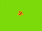
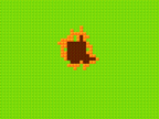
Instead changing to some specific state based on the surrounding states, you can change to any state with some probability. These probabilities depend on the surrounding states, and can possibly be zero.
 |
 |
 |
 |
 |
 |
 |
 |
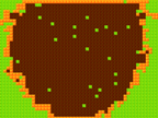 |
Adding probability to the mix can have several advantages:
It introduces variability in patterns. This means a specific (perhaps the start-up pattern) will not always produce the same results.
It can enhance the organic look of the system. Cross and squares patterns are common in deterministic CA systems. For many purposes, this is unsatisfactory (have you ever seen a fire spreading as a growing square?) Adding probabilistic state changes will make the patterns more organic and varied.
It can make discreet behaviour more continuous. For example, two common “problems” with CA systems are exponential growth (where all cells go to a certain state outwards very quickly), or sudden death (where all cells go to a certain state very quickly inwards). The problem is often that a single change in the update rules results in a exponential growth system to become a sudden death system, with seemingly no way to get a “sweet spot”. If states can only change with a certain probability, tweaking the probabilities allows you to get intermediate patterns (stable growth, equilibrium, or stable death).
It allows you to control the speed of the simulation. It is especially helpful to slow down a simulation without making it more granular (in the time dimension). It is useful to multiply all your probabilities with a global parameter that you can tweak to control the speed.
Note that in the example above, certain cells did not burn at all – per chance, they did not caught fire when their neighbours were burning. Timers (see below) can reduce or eliminate this effect.
Adding randomness can increase the emergence, and hence also unwanted emergence, so care must be taken that the simulation is always valid.
Tile Interpolation
 |
 |
 |
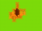
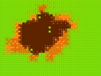
Normally, you want your simulation to be as simple as possible. However, when such simple simulations are displayed (visualised), the results can be unsatisfactory. One way to get better visual quality is to use tile (cell) interpolation to make the simulation seem more complicated than it really is. When combined with a bit of randomisation, the effects can be very convincing.
The basic idea is to simulate only every nth cell with the CA approach. Other cells are interpolated. The number of interpolated cells can be adjusted, depending on the detail level required (balanced with the combinatorial number of tiles required!)
In the fire simulation, using only three states makes the simulation seem very primitive. Suppose that we simulate only every second row, and in these, only every second column, and fill the remaining cells depending on their neighbours. We have to create a function that will return a tile for each combination of surrounding tiles:
get_center_tile(north, east, south, west)
Interpolation rules are similar to update rules of the simulation, and hence can easily be as complicated. If this is the case, you would do better to implement more states and not do any interpolation. Interpolation should only be used if it significantly reduces the implementation complexity.
Timers
 |
 |
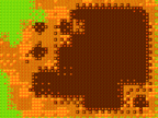 |
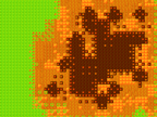
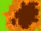
Some interesting effects can be obtained if each cell has a timer, that is, each cell only updates once the timer expires. Some rule determines when the timer is reset. For instance, the timer can be set:
- randomly,
- as a function of the state,
- as a function of the surrounding cells,
- as a function of another property of the tile (*1),
- as a function of some external process (*2).
(*1) For instance, if each cell has an associated “burning capacity” parameter, (simulating material types), a fire state timer can be set in proportion to this parameter.
(*2) For example, we can set timers according to a wind factor.
Timers can have the following effects:
- add some randomness to a simulation,
- slow the simulation down,
- smear the simulation (for example, in the fire simulation, the burning border is much thicker, and no cells are skipped).
Although you can often implement your grid cells as classes (or structs, or whatever aggregating construct your language provides) with states and timers embedded, it is simpler (on more efficient) to have separate integer grids – one for states and one for timers.
Note that if timers do not have the same expiration time, you the CA system is asynchronous and the behaviour can differ dramatically from a synchronous CA system. Thus, you should include timers early in the development process, so that their effect does not force you to re-tweak all the parameters.
If your world is big, you cannot run the CA for the whole world at every time step – it will kill performance. Below are some ideas for improving performance.
Instead of simulating the entire world, you can only simulate the part that is relevant to the game, usually the visible region of the game. A simple technique is to use a wrapped grid, similar to the grids used for the visual port in scrollable 2D games. This grid can be slightly larger than the visible grid, so that it allows cells to update naturally for a few iterations before they become visible, and so increase the illusion of a persistent world.
To hide that fact that you are only simulating a very small piece of the world, you must update “new” cells appropriately. There are several options:
Update cells to a natural starting state. In many cases, this solution is adequate, especially if you simulate a slightly larger grid than is visible.
Copy states from the existing simulation. Here you can copy neighbouring cells, or randomly from a nearby region. Copying from nearby cells promotes spatial coherence.
Initialise states statistically. Based on a neighbourhood of cells, each cell is initialised probabilistically. For example, each cell can be initialised randomly to one of three neighbouring cell’s states.
Use hierarchical modelling. Use another CA system that represents the entire world in very low detail, and use this to initialise the cells of the high detail version. Note that both the states and the update rules will differ for the high and low detail simulations. Use probabilities to prevent homogeneous systems. You can even use several levels of detail, and incorporate them as needed. Beware the extra implementation complexity, though!
This technique does not work when the world is should be changed permanently.
Instead of only simulating a part of the world, you can only update a part of the world. This requires enough memory for the whole world, but only processing power for the cells you wish to update. This method has the advantage of real persistence, thus permanent changes can be reliably simulated. Which cells you update will determine how your simulation will play out:
- Update all visible cells (or a slightly larger region). This is the most natural update scheme, and its effects are similar to partial simulation described above.
- Divide the world into discontiguous regions, and update a different region each time step. For example, divide the world into two sets: one contains every other cell, the other the rest, and update these two sets alternately. To save a significant amount of processing, you need many sets. To hide patterns in the updates that might break the illusion of a continuous world, the sets should be irregular. This method has the advantage that real things happen off screen. On the down side, it slows down the simulation significantly.
- Combine the two methods above.
Partial updating, like the inclusion of timers, lead to an asynchronous system, and hence the behaviour might be very different from that of a fully updated system.
In certain cases, simulations can be baked offline and be used in games. This means you perform the simulation before the time, and record each frame. The game then reads these frames, and plays them back.
Various schemes are possible to get more with less. For instance, you can also interpolate the simulation in time. With some thought, you can simulate events in a way that they can be looped, stacked together, and started and stopped unobtrusively. This means you can blend them with the interaction in a way that will not make it obvious that the simulation has been performed off-line.
Unwanted Emergence
Not all emergence is good, and you might find it hard to prevent certain behaviours. If the unwanted behaviour is only visual, and it occurs only rarely, it might be acceptable. However, if behaviour impacts play negatively, it must be prevented.
As with all tweaking, you should not spend too much time fumbling around. To proceed more “scientifically”, ask yourself the following questions:
- Is there a way to detect (measure objectively) the unwanted behaviour?
- Instead of tweaking your CA, can you detect-and-recover system be used?
- Is the behaviour continuous? In other words, is there a degree of badness, or is it either good or bad?
- If it is continuous, is it feasible to kick in a preventative system? (When the badness goes above a threshold, updates are processed differently).
- Is it feasible to find a set of parameters through an optimisation algorithm (for instance, genetic programming)? It might even be possible to search exhaustively for a solution.
- Is my model too complex? Try to eliminate states and simplify transition rules. You might even consider breaking your simulation into two or more independent CA systems.
- If you find yourself struggling to tweak the parameters for too long, you should perhaps look for a better model that is less sensitive to the exact parameters.
Links
Online Demo
http://blog.soulwire.co.uk/laboratory/flash/2d-cellular-automata Browswer-based demo with ActionScript source code.
General
http://cell-auto.com/ A nice breakdown of various topics related to Cellular Automata. The article on optimisation is especially interesting.
http://www.collidoscope.com/modernca/ Contains many non-traditional variations of cellular automata.
http://www.fourmilab.ch/cellab/ Application for exploring cellular automata.
Applications and Implementation
http://realtimecollisiondetection.net/blog/?p=57 Path finding using cellular automata.
http://www.ibm.com/developerworks/java/library/j-camusic/ Cellular Automata and music (interesting way of creating procedural music).
http://blog.sigfpe.com/2006/12/evaluating-cellular-automata-is.html About using lazy, infinite containers for cellular automata.
http://madeira.cc.hokudai.ac.jp/RD/takai/automa.html Graphics applications for cellular automata – lots of videos!
Game Design
http://www.gamestudies.org/0102/pearce/ An article about game design.
http://www.cp.eng.chula.ac.th/~vishnu/gameResearch/Sweetser_Thesis.pdf A thesis that looks at game design from a emergence perspective.
http://fora.tv/2006/06/26/Will_Wright_and_Brian_Eno#chapter_01 Will Wright and Brian Eno on generative systems.
Downloads
Game Maker Demos
- Requires Game Maker 7.
- Contains 9 demos.
ca_demos.zip (135 KB)
interesting. i’m working on a city simulation game using Game Maker and have been interested in CA for a while now. the downloaded files were interesting and its nice to see a demonstration of CA that works with a program i understand already like GM
Cities are very interesting systems to simulate. Do use use CAs in your simulation?
ht
interesting…..i am interesting in CA i want learn more pleas i need your advice , to improve myself ….. specially in city simulation ….your reply highly appreciated …