For many applications, detailed statistical models are overkill. Instead, we can get away with a rough description of the distribution – not in mathematical formula form, but just as a graph with a few sample points.
For example, when trying to model the traffic around a school, you might know that the graph looks something like this:
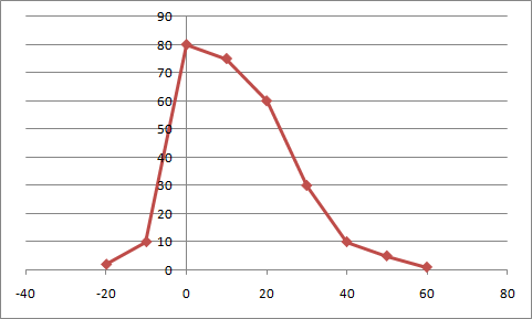
The input is the number of minutes before the first bell rings, and the output the number of children dropped off at that time. You know that most kids are brought before the bell rings, and that the closer to the bell, the more kids are being brought every minute. Only a few kids are late.
This tutorial describes how to generate random numbers that can generate a distribution described by an arbitrary (piece-wise linear) curve, as the one above.
Implementation
1. Calculate an accumulative probability
The first step is to run an accumulative sum of our original sample points. The following code snippet shows how it can be done in C++; the array “samples” contains the original samples.
for(int i = 1; i < n; i++)
{
    samples[i] += samples[i - 1];
}
The snippet above does the calculations in-place, but it is not necessary, as is shown in the snippet below:
newSamples[0] = samples[0];

for(int i = 1; i < n; i++)
{
    newSamples[i] = samples[i] + newSamples[i - 1];
}
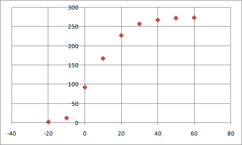 The graph above shows the accumulative probability density.
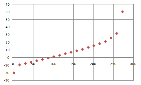
2. Calculate inverse sample points
This step is easy – we simply swap the input and output samples. It is not necessary to do this explicitly, just swap them in the argument list of the function call in the next step. 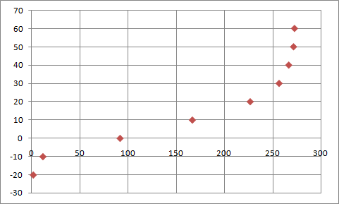
3. Interpolate between samples
I use a special data structure that makes it very easy to compute the interpolations from discreet sample points: the response curve. There are two varieties. The ordinary response curve, with uniformly spaced samples, and the xy-response curve, where samples can be arbitrarily spaced. 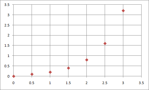 Ordinary Response Curve.
 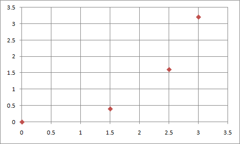 XY-Response Curve. The implementation is very simple, so I won’t describe it here. A C++ implementation is available in the Special Numbers Library; a Python implementation is available with the example below. Here I simply explain the usage as it relates to this tutorial. We proceed as follows:
- First, we construct an xy-response curve from our samples of the inverse accumulative probability.
- Then we sample this curve at regular intervals, and load it into a ordinary response curve (we do this, simply because the ordinary response curve is much faster than the xy-version).
//...
int oldSampleCount = 7;
int newSampleCount = 20;

float inputMin = 0.0f;
float inputMax = 3.2f;

//note: input and output is swopped arround, because we want the inverse!
XYResponseCurve<float, oldSampleCount> xyCurve(outputSamples, inputSamples);
for(int i = 0; i < newSampleCount; i++)
{
input = ((float) i / (newSampleCount - 1)) * (inputMax - inputMin) + inputMin;
uniformOutput[i] = xyCurve(input);
}
ResponseCurve<float, newSampleCount> curve(inputMin, inputMax, uniformOutput);
4. Map uniform random numbers to the input range of the IAPDF, and calculate the output
Now that we have the response curve, we can map uniform random numbers to the appropriate input range. For the example above, we need to map to the range [0, 3.2]. The snippet below shows how to generate random numbers with the distribution shown above:
//...create the curve c
float input = random(); //Uniformly distributed function between 0 and 1.
float scaledInput = r * (inputMax - inputMin) + inputMin;
float output = curve(scaledInput);
The graph below shows how 10 000 random numbers are distributed. It follows the original graph closely; the discrepancy at -10 is caused by the way samples are counted (all samples between -10 (inclusive) and 0 (exclusive) are counted and plotted at -10. 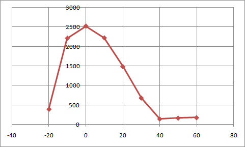
Tips and Pitfalls to Avoid
- Generate sequences for all intermediary steps.
- Use Excel, Calc, or some other spread sheet program to debug these sequences visually when things go wrong.
- It is very easy to get confused with input, and output, especially after the swap. Watch out for this!
- It is easy to get confused with the number of samples for the various sequences.
- If you implement your own Response Curve data structure, unit tests will save you huge amounts of time.
- Always make sure that you sample enough points, especially if your original distribution graph has rapid changes in it.
- Always confirm that your random output follows the distribution you wanted.
- It might be faster to use this method even when mathematical formulas are available.
Downloads
Example C++ Source Code
http://code-spot.co.za/downloads/cpp_examples/arbitrary_distribution.cpp Requires Special Numbers Library
Example Python Source Code
http://code-spot.co.za/downloads/python_examples/random_distributions.py
Comments