It is sometimes necessary to find the distribution given a sample set from that distribution. If we do not know anything about the distribution, we cannot recover it exactly, so here we look at ways of finding a (discrete) approximation.
I will cover the case for 2D sets here, but the ideas are easily extended to any dimension.
Visual Inspection From a Scatter Plot
The easy way to estimate the distribution is to simply look at a scatter plot of the samples.
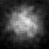
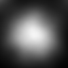
| A scatter plot of a 2D sample set. (A pixel was simply drawn at each point of the sample. The images was slightly blurred to give the pixels more substance).Here we can already estimate the distribution, as we can intuitively “see” the shape. | |
If the distribution is simple, we can often “guess” suitable parameters for a mathematical function. But this method is not suitable when more accuracy is required. And obviously this method does not work for higher dimensions.
I always use a visual inspection as a first step when using the other methods described here. First, it allows you to decide which approach to use. Second, it serves as a rough benchmark to test the results of a better method against.
Averaging Over a Grid
For this method, we divide the domain in cells, and count the number of points in each cell. To normalise, we divide the counts by the total number of points to get a distribution.
Typically, we choose a cell size large enough so that all cells contain a few points.
It is possible to use different cell sizes, so that regions of higher density has more cells, for instance, by using a quad tree. However, this approach makes it difficult to interpret the values (they should be scaled down by a factor of the area they represent), and to generate random numbers from this distribution. I can’t really imagine a situation where this approach will be preferred above using a regular grid or convolution.
Convolution
There are two ways to implement convolution. The first should be used when the sample set is small relative to the size of the domain, otherwise the second method will be more efficient.
Sparse Point Convolution
Generate a very granular empty grid over the domain.
For each point p in the sample set,
- map p to the grid (calculate the coordinates x,y of p in the grid),
- add a number to all the cells in the neighbourhood of p in the grid.
Now normalise the grid.
The neighbourhood is typically a circle or a square. The number you add can be the same for all neighbours (in which case any positive number will do), or it can be scaled depending on the distance from p.
The size of the neighbourhood depends on the density of your sample. In general, the denser it is, the smaller the neighbourhood can be. Smaller neighbourhoods lead to faster execution. To prevent “holes” in the approximation, use a radius that corresponds to the maximum of the distances between a point and its closest neighbour.
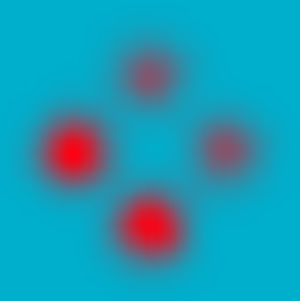 |
 Estimation with a constant square neighbourhood. Estimation with a constant square neighbourhood. |
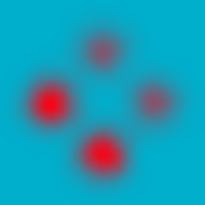 |
 Estimation with a constant circular neighbourhood. |
 |
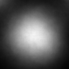
 Estimation with a circular neighbourhood with a falloff. |
Traditional Convolution
Generate a very granular empty grid over the domain.
For each point p in the sample set, map p to the grid (calculate the coordinates x,y of p in the grid), and add one to that location in the grid.
Now choose a square, symmetrical convolution matrix, and perform a discrete convolution on the grid:
new_grid[i, j] = sum_{i,j} grid[i][j] * c[i][j]
Here the i, j go over the indices of the convolution matrix. (Normally, the convolution is defined as new_grid[i, j] = sum_{i,j} grid[n – i][n – j] * c[i][j]. However, since we are suing a symmetrical matrix, these definitions are equivalent, and we need not perform the extra calculation).
Now normalise the grid.
The convolution can be a square or circle of 1s, or be filled with numbers that grow smaller outwards. These correspond to the three neighbourhoods described for the sparse convolution.
Note that the new_grid is larger than the original by one less than the size of the convolution matrix in each dimension. The centre of the new grid corresponds with the original grid.
For example, if the original grid was 100×100, and the convolution matrix was 5×5, the new grid will be 104×104. The point (2, 2) in the new grid corresponds to point (0, 0) in the original grid.
About Normalisation
It is customary to normalise the distribution so that all the probabilities add to 1. But for many purposes we need only relative probabilities, and this step can be skipped. For example, the method of generating random numbers described in a previous post uses only relative probabilities.
A Few Tips
- Always test your distribution by generating a random set from it, and comparing it with the original sample. They should match qualitatively.
- The smaller your sample set, the cruder the approximation should be. That is, cells, neighbourhoods or convolution matrices should be big. There is a limit to the accuracy you can obtain from any sample – if you try to exceed it, your results will be poor.
- The most common implementation errors are made at the borders (of any grid or matrix) – watch out for them!
Download
There is an example of implementation in 2D in with the Python Image Code. See the file random_distributions_demo.py.